Correction Of The Sample Rate Of The Sample Distribution With Standard Errors

PC running slow?

1. Download ASR Pro from the website

2. Install it on your computer

3. Run the scan to find any malware or virus that might be lurking in your system

Improve the speed of your computer today by downloading this software - it will fix your PC problems.

In this guide, we are going to identify some potential causes that can affect the sample distribution standard fraction of the sample distribution, and then I will suggest some possible fixes that you can try to fix this problem. Standard error (SE) associated with sample proportion: √ (p (1-p) n). Note: The standard error usually decreases with increasing sample size.

• Behavior in relation to the proportions of the sample.
• Approximate distribution of the sample proportion.

CO-6. Apply the basic concepts of probability, chance Variance and commonly used statistical probability distributions.

Proportions Of Behavior Patterns

EU 6.21: Use sample proportion when choosing distribution (if applicable). In particular, you must be able to identify exceptional specimens from a specific population.

• The unexpected distribution of the proportions of samples (p-hat) into duplicate samples (of the same size) is known as marketing p-hat sample.

The goal of the following video exercise is to ensure that information about the center, distribution, and shape of the sample distribution comes from the p-hat through reconstruction simulations.

At this point, we have a great idea of ​​what happens when we confirm random samples from the population. Our simulator assumes that our initial guess about your current shape and center of the pattern is correct. If there is a good proportion of p in the general population, then random samples of the same type from the general population also have the proportions of the sample p. What’s even more dangerous is that selectivethe distribution of proportions has an average value of p.

We also figured out why in this situation the proportions of the samples are approximately normal. We will see later that this is not always the case. But although the proportions of the sample are distributed normally, part of the distribution is concentrated on p.

We now want you to be able to use simulation to help us think about the expected variability in sample ratios. Our intuition tells us that larger samples cover the population roughly better, so we can expect even less variability with larger samples.

In the next run, we will use simulation to explore this important idea. After this passage, we will link these ideas to a more formal theory.

Amplified models are appropriate for our information. Larger random samples will give a better idea of ​​your proportion of the population. If the sample is now large, the proportions of the sample will decrease to p. In other words, with larger samples, the distribution of samples is less volatile. Advanced probability theory confirms our observations and benefits. provides a much more accurate way of describing the current change in sample ratios. This is described below.

Selective Proportion Related To Distribution

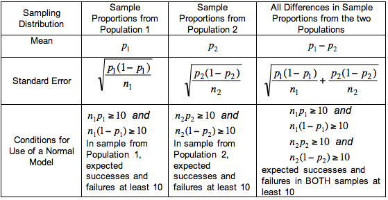
If repeated random samples are drawn for a categorical variable with respect to a given variable n from a value society where exactly the proportion in the observation category is p, then the mean of all sample dimensions (p -hat) is the percentage of the population (p).

Regarding the distribution of all sets of samples, the theory dictates the behavior of one much more accurately than the statement that for large samples the multiplication is less. In fact, the reference deviation of sample proportions is directly related to sample size, as classified below.

Since the sample size n is related to the square root of the denominator, the standard deviation decreases as the sample size increases. Finally, the exact shape of the p-hat distribution remains roughly normal as long as the size of the n-test is large enough. By convention, np and n (1 – p) must be at least 10.

Let’s apply this result to eachSee the next example and see how it compares to our simulation.

In our example, n = 25 size) (sample and p = 0.6. Note that np = 8 10 p) and n (1 = ten ¥ 10. Thus, we can infer that p- the hat will be about the level of the normal distribution with a mean p = 0.6 standard and deviation

(which is very similar to what we saw in our simulation).

• These good results are similar to those for the known binomial variables (X) described above. Be careful not to confuse the results and the mean standard deviation of X with p-hat people.

When forming a sample distribution, we can usually apply the standard deviation rule and use z-scores to describe probabilities. Let’s take a look at a few examples.

To examine the effect of sample size on the likelihood of these calculations, consider the following modification to our example.

• As long as the trial is truly random, the p-hat distribution can be described as centered on p, regardless of the size of the experiment. Larger o Samples have not received such wide distribution. In particular, if we multiply the structure size by 25 and increase it from 150 to 2500, the standard deviation decreases to 1/5 of the original standard modification. The sample share deviates less from the zero population share. If 6, then the sample is larger: it tends to decrease from 0.5 to 0.7 for samples of size 100 and tends to decrease between 0.58 and 0.62 for samples of size 2500. This does not mean that the true value is only 0.56 for 100 related samples (greater than 20% probability), but it is almost impossible to state a value of just 0. For sixty out of 2500 samples (almost zero probability).

EXAMPLE 6: Behavior Of Aspect Patterns

About 60% of part-time students in the US tend to be women. Other (expressed in words, the percentage of women among part-time students is p = 0.6). What can be expected in terms of the behavior of each proportion of women in the sample (p-hat) if the random sample, sample size 100 is far from the population of all part-time college or university students A day?

As we saw earlier, due to sample variation, the sample share in random samples of size 100 takes on numerical values ​​that can vary according to the laws of randomness: in other words, the sample share is arbitrarily large. To summarize the behavior of any unbound variable, let’s focus on three characteristics associated with its distribution: center, general spread, and shape.

Medium: Some samples are in the low tier, such as 0.55 or 0.58, while others are in the uppermost, such as 0.61 or 0.66. It is reasonable to expect that each of the proportions in the sample will average over the base fraction of the number 0 in a repeated random sample. 6. In other words, the mandatory reference to the p-hat distribution should be p.

Distribution: for products out of 100, we expect that the sample rates for women will not differ significantly from the population share of 0.6 at the same time. Sample sizes smaller than 0.5 or larger than 0.7 would be quite unexpected. On the other hand, if we only take a dish of size 10, we will not be automatically surprised even by this a small sample of women, mainly because 4/1 0 = 0.4, sort of or better, although 8/10 = 0.8. Hence, the sample size plays a role in the variance of the sample proportion reproduction: for large samples there should be less variance, for smaller samples there should be more variance.

Shape: Sample proportions close to 0.6 should probably be the most common, and sample proportions well above 0.6 in both directions will certainly be increasingly unlikely. In other words, the shape of the person’s distribution should bulge out in the middle and merge at the ends: it should become somewhat normal.

EXAMPLE 7: Using A Distribution Pattern Pointing To P-hat

A random sample of 100 students was drawn from all part-time students in the United States, where the overall proportion of women is 0.6.

(a) Between which pair of values ​​(p-hat) is there a 95% chance that the share of experience is?

First of all, notice that the p-hat distribution is complete with mean p = 0.6, standard deviation

and the form you cano call normal, 100 (0, because np =. = 6) 59 and n (1 – p) = 100 (0.4) = If 58 both are greater than 10 The standard deviation rule is true: probability relative to 0.95 addition that p-hat is within 2 standard deviations depends on the mean, that is, between 0.6–2 (0.05) and 0.6 + 2 (0.05). The probability that the p-hat will fall is about 95% using the sampling interval (0.5, 0.7) of this sizing guideline.

(b) What is the probability that the proportion of the sample p-hat is less than or equal to 0.56?

We will normalize 0.56 of your Z-score by subtracting the mean and dividing the highest score by the standard deviation. We can then determine the probability using an erogenous rate calculator or table. 8: C

Sample Distribution Of A Sample Associated With P-hat

Our part-time students from most of the United States were randomly selected from 2,500 students, with a total female rate of 0.6.

(a) There is always a 95% chance that the proportion of the sample (p-hat) is between which values?

The first note for which the p distribution has a mean p = 0.6, offloning

and usually a form that approaches normal, since np = 2500 (0.6) = Et n (1 fifteen cents – p) = 2500 (0.4) = 1000 both are much greater than 10. Correlated standard deviation rule: probability that p-hat is within 2 standard deviations of the input, that is, H. between 0.6-2 (0.01) and 0.6 + 2 (0.01). The probability that the p-hat will appear in all samples (range 0 58, 0.62) for this size in turn is about 95%.

(b) What is the probability that the sample for the p-hat test is less than or equal to 0.56?

We normalize 0.56 to one by subtracting the mean and dividing the feed by the standard deviation. Then we will most likely find the probability with a car or a normal normal table.

Improve the speed of your computer today by downloading this software - it will fix your PC problems.

Korekta Częstotliwości Próbkowania W Stosunku Do Rozkładu Próby Z Błędami Standardowymi
Correção Da Taxa De Ajuste Da Distribuição Da Amostra Com Erros Clássicos
Correzione Del Track Rate Della Distribuzione Del Campione Con Errori Impostati
Correctie Met Betrekking Tot De Steekproeffrequentie Van De Voorbeeldinzendingen Met Standaardfouten
Corrección Del Precio De Venta De Muestra De La Distribución De Muestra Con Errores Estándar
Correction Du Taux De Groupe De La Distribution De L’échantillon Avec Des Erreurs Familières
Корректировка выборочной потребности выборочного распределения со стандартными ошибками
Korrektur Der Samplerate In Verbindung Mit Der Sampleverteilung Mit Standardfehlern
광범위한 오류가 있는 표본 분포의 표본 비율 수정
Korrigering Av Samplingsfrekvensen Avseende Provfördelningen Med Standardfel